Experiments with Postgis2.0 rasters

These are  my notes on understanding/evaluating raster support in Postgis 2.0 .

Platform

  • Windows 7
  • PostgreSQL9.0
  • Postgis2.0


Key Resources

  1. Installation on Windows:
    Jorge Arevalo’s notes
    are key. (But expect ‘minor’ variations based on your own system’s configurations, esp. with gdal)
  2. Loading rasters into postgis tables and getting some understanding of it
  3. Working with postgis raster: intersections with vector datasets

1. Example data i used

  • SRTM for southern India downloaded from here, clipped in QGIS using gdaltools plugin, called srtm_clip.tif
  • A vector layer i had of administrative boundaries, called wards

2. Loading an elevation raster into Postgis2.0

a. Using raster2pgsql.py, in a command line, like so:

raster2pgsql.py -r srtm_clip.tif -s 4326 -I -t srtm_table -k 700×700 -o srtm_clip.sql

where

  • srtm_clip.tif is the input elevation raster
  • 4326 is the EPSG code for lat-long, wgs 84 coordinate system
  • -I tells it to make a spatial index
  • -k 700×700 is the size of each tile to break the input raster into
  • srtm_sql is the output file that will contain the sql commands that creates the raster table in the database that has previously been set up

b.Load the sql file

Use pgAdminIII’s sql editor to open the ‘srtm_clip.sql’ the above step created, and run it.

FYI this is what the generated sql file looked like. (and i could not get the psql command line option for loading the sql file to work). It ran in less than a second.

BEGIN;
CREATE TABLE “public”.”srtm_table” (rid serial PRIMARY KEY);
SELECT AddRasterColumn(‘public’,’srtm_table’,’rast’,4326, ARRAY[’16BSI’], false, true, null, 0.000833333333333, -0.000833333333333, 700, 700, ST_Envelope(ST_SetSRID(‘POLYGON((77.256195534800000 13.681944121300001,77.256195534800000 12.561944121300002,78.131195534800000 13.681944121300001,78.131195534800000 12.561944121300002,77.256195534800000 13.681944121300001))’::geometry, 4326)));
INSERT INTO “public”.”srtm_table” ( rast ) VALUES ( (‘01000001004F1BE8….’)::raster );
CREATE INDEX “srtm_table_rast_gist_idx” ON “public”.”srtm_table” USING GIST (st_convexhull(rast));
END;

c. What do you get?

  • Refresh the database and you’ll see a new table called srtm_table.
  • It has two columns rid and rast, and 4 rows. each row is for a rid, which i guess is a tile id.
  • Each rid references one tile – choosing k=700×700 caused the input raster to be split into 4 tiles
  • Smaller tiles are generally better – but i did run into one issue (you’ll see in just a bit)

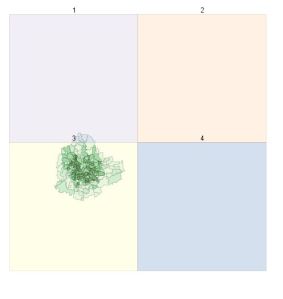
Viewing the tiles (in OpenJump, because Qgis 1.6 does not work with Postgis2.0, even for non-rasters).

4 srtm tiles (overlaid over administrative boundaries)

  • Useful commands at this point

— postgis versions
select postgis_full_version(), postgis_raster_lib_build_date(), postgis_raster_lib_version();

— raster formats
SELECT short_name, long_name
FROM st_gdaldrivers();

–metadata
SELECT (md).*, (bmd).*
FROM (SELECT ST_Metadata(rast) AS md,
ST_BandMetadata(rast) AS bmd
FROM srtm_table LIMIT 1
) foo;
— no data value was not set even though i did put it into the QGIS-gdal plugin application

–size
SELECT pg_size_pretty(pg_total_relation_size(‘srtm_table’));
–gives 1.8mb

–no-data value setting
UPDATE srtm_table SET rast = ST_SetBandNoDataValue(rast,-32768);
vacuum analyze srtm_table;

–summary stats (mean) of the raster

SELECT ST_Quantile(rast, 0.5) As value
FROM srtm_table;
— this seems to give me the median of each rid (but i want the median of the entire raster)

1;886
2;339
3;857
4;0

2. Intersecting raster with vector layers

a. performing the intersection

This below worked, creating 70,503 rows – but it took 80 minutes!!!

create table srtm_wards_inter as
select
ward_name,ward_id, (gv).geom As the_geom,(gv).val
FROM (Select ward_name, ward_id,ST_Intersection(rast,geom) As gv
From srtm_table, wardscleanattributes
WHERE geom && rast
and ST_Intersects(rast, geom)) foo;

b. extracting area-weighted mean elevations per ward polygon (sorted by mean elevation)

 SELECT ward_id,ward_name,
sum(ST_Area(ST_Transform(the_geom, 32643)) * val) /
sum(ST_Area(ST_Transform(the_geom, 32643))) AS meanelev
FROM srtm_wards_inter
GROUP BY ward_id, ward_name
ORDER BY meanelev, ward_id;

–gives me the ward id’s, names and mean elevations for all 198 wards

159;”Kengeri”;792.638912308088
131;”Nayandahalli”;821.362355078139
130;”Ullalu”;828.12323070928
198;”Hemmigepura”;831.628739711782

67;”Nagapura”;921.610375368031
46;”Jayachamarajendra Nagar”;922.392379372865
179;”Shakambarinagar”;922.91608088907
62;”Ramaswamy Palya”;923.071218071726
9;”Vidyaranyapura”;923.304108544661
16;”Jalahalli”;924.921270389213
63;”Jayamahal”;926.957157345059
93;”Vasanthnagar”;928.315490103474
194;”Gottigere”;931.443435808278
34;”Gangenahalli”;932.719869810253
45;”Malleshwaram”;932.814742613641
35;”Aramanenagar”;935.117666378835

Major Questions

      1. Why did the intersection take so long (see 2a above)
      2. How can i get raster statistics irrespective of rid?
          1. example: quantile stats for the raster are split by rid (i.e tile)
          2. example: if i get median elevation by ward like so:
            1. SELECT ward_id,ward_name,ST_Quantile(rast,0.5) As median
                  FROM srtm_table,wardscleanattributes
                      WHERE ST_Intersects(rast,geom)
              ORDER BY ward_id, median;

I STILL get multiple entries per ward, if (i) the ward crosses two or more rid (tiles), or (ii) the ward is split into 2 polygons

If anyone can help with the above, I can update my post soon.
Thanks!
Comments (1)

GHCN data in a Postgis database

Goal

I’m continuing my experiments with postgresql/postgis databases, using the Global Historical Climate Network (GHCN v2)  dataset of monthly precipitation and temperature data from around the world. I’m going to create and query a database out of GHCN data, downloaded here on May 4, 2010.

Tips

Read the metadata on the site, because the format is a bit tedious.The main things to note are:

  • i had to convert the station list table v2.precip.inv to a csv file before i could copy it into a postgres table
  • i had to import the ~80Mb datafile (v2.prcp) as a postgres table of text rows, and then parse the actual columns out (see sql below) into a new table
  • the code in the stations list table has one digit less than that in the data table – a code for whether there are data duplicates or not (read the metadata file online)
  • i’ve used the raw data here. there is a separate quality-controlled table of data that is MUCH smaller – i have not used that here.
  • -9999 represents null data, -8888 respresents trace precipitation

Code

–create GHCN station table

— drop table ghcn_stations;

create table ghcn_stations (code numeric primary key not null, name varchar(40), country varchar(25), latitude float, longitude float, elevation integer) with OIDS;

–load from text file

copy ghcn_stations FROM ‘E:/gisdata/World/GHCNv2/v2.prcp.inv.csv’ CSV;

–select stations in Uganda

select * from ghcn_stations where country = ‘UGANDA’;

–make a geometry column out of lat and longitude

Alter table ghcn_stations add column the_geom geometry;

–populate with lat and long and 4326 srid

Update ghcn_stations

SET the_geom = PointFromText(‘Point(‘||longitude||”||latitude||’)’,4326);

–above did not work

Update ghcn_stations

SET the_geom = ST_Point(longitude,latitude);

–above worked but srid not yet set

Update ghcn_stations

SET the_geom = St_SETSRID(the_geom,4326);

–above set the SRID

–now add spatial index

create index idx_ghcn_stations on ghcn_stations using GIST(the_geom);

VACUUM ANALYZE;

–test out how to extract select characters from a numeric field, below worked

select country, substring(cast(code as text) from 1 for 5)) from ghcn_stations

where country = ‘UGANDA’ OR country = ‘TANZANIA’ or country = ‘KENYA’;

–load from text file

copy precip FROM ‘E:/gisdata/World/GHCNv2/v2.prcp.csv’;

–does not work well, reading each line as one long text string

–also could not load big file in excel to convert to csv

–so tried reading it as individual text lines to parse later

select * from precip limit 5;

select substring(codeyr from 1 for 16) from precip limit 10;–this extracts the station code and year i.e. column1

select substring(codeyr from 17 for 5)::numeric from precip limit 100;–this extracts i think the month of jan

select substring(codeyr from 22 for 5)::numeric from precip limit 100;–this extracts i think the month of feb

select substring(codeyr from 27 for 5)::numeric from precip limit 100;–this extracts i think the month of mar

select substring(codeyr from 32 for 5)::numeric from precip limit 100;–this extracts i think the month of apr

select substring(codeyr from 37 for 5)::numeric from precip limit 100;–this extracts i think the month of may

select substring(codeyr from 42 for 5)::numeric from precip limit 100;–this extracts i think the month of jun

select substring(codeyr from 47 for 5)::numeric from precip limit 100;–this extracts i think the month of july

select substring(codeyr from 52 for 5)::numeric from precip limit 100;–this extracts i think the month of aug

select substring(codeyr from 57 for 5)::numeric from precip limit 100;–this extracts i think the month of sep

select substring(codeyr from 62 for 5)::numeric from precip limit 100;–this extracts i think the month of oct

select substring(codeyr from 67 for 5)::numeric from precip limit 100;–this extracts i think the month of nov

select substring(codeyr from 72 for 5)::numeric from precip limit 100;–this extracts i think the month of dec

— so now create a new table with the data parsed right

create table newprecip as

select substring(codeyr from 1 for 11)::numeric as code,

substring(codeyr from 12 for 1)::integer as duplicates,

substring(codeyr from 13 for 4)::integer as year,

substring(codeyr from 17 for 5)::integer as m1,

substring(codeyr from 22 for 5)::integer as m2,

substring(codeyr from 27 for 5)::integer as m3,

substring(codeyr from 32 for 5)::integer as m4,

substring(codeyr from 37 for 5)::integer as m5,

substring(codeyr from 42 for 5)::integer as m6,

substring(codeyr from 47 for 5)::integer as m7,

substring(codeyr from 52 for 5)::integer as m8,

substring(codeyr from 57 for 5)::integer as m9,

substring(codeyr from 62 for 5)::integer as m10,

substring(codeyr from 67 for 5)::integer as m11,

substring(codeyr from 72 for 5)::integer as m12

from precip

;

–check first 12 rows, looks ok

select * from newprecip limit 12;

code|duplicates|year|m1|m2|m3|m4|m5|m6|m7|m8|m9|m10|m11|m12|gid
20743086004|1|1962|0|0|0|833|0|663|3005|1658|2470|419|548|786|1
20743086004|1|1963|0|0|0|-9999|-9999|-9999|1061|2422|-9999|736|0|0|2
20743086004|1|1964|0|0|0|0|0|971|-9999|1963|-9999|86|20|0|3
20743086004|1|1965|0|0|38|84|0|450|2039|1397|1896|0|0|0|4
20743086004|1|1966|1194|0|30|73|128|1011|5265|2544|3710|981|780|240|5
20743086004|1|1967|60|0|380|0|0|2020|3310|2161|1641|0|0|887|6
20743086004|1|1968|340|150|10|30|100|1046|3319|893|2096|729|70|60|7
20743086004|1|1969|330|0|30|0|270|1100|2209|1647|3933|140|150|160|8
20743086004|1|1970|215|0|-9999|40|520|2014|1325|1734|1748|116|0|0|9
20743086005|1|1951|0|0|610|38|259|1473|2974|2136|1186|424|0|0|10
20743086005|1|1952|155|0|10|107|102|889|2532|1994|2624|396|0|0|11
20743086005|1|1953|165|0|0|356|0|4389|3406|5570|3129|922|0|0|12

— add primary key note that it needs to be unique so i have to add a serial first

alter table newprecip add column gid serial not null;

create unique index uidx_newprecip_gid on newprecip using btree(gid);

alter table newprecip add constraint

pkey__newprecip_code PRIMARY KEY(gid);

–try out some select queries like extracting data for Masaka, Uganda

select newprecip.*, ghcn_stations.name, ghcn_stations.code

from

ghcn_stations join newprecip

on ghcn_stations.code = newprecip.code

where ghcn_stations.country = ‘UGANDA’

order by name;

–lets try and extract the min and max year of available data

select ghcn_stations.name,min(newprecip.year) as minyr, max(newprecip.year) as maxyr

from newprecip, ghcn_stations

where ghcn_stations.country = ‘UGANDA’

and newprecip.code = ghcn_stations.code

group by ghcn_stations.name

order by maxyr DESC, name;

— but MASAKA in Uganda does not appear in this list…why?

— maybe the codes in the 2 tables that i use to join above dont match?

select ghcn_stations.code as code1

from ghcn_stations

where ghcn_stations.name= ‘MASAKA’;

select * from ghcn_stations

where name = ‘MASAKA’;

— both of the above find Masaka

— BUT the country name is missing for MASAKA in the ghcn_stations table

— so lets add it

update ghcn_stations

set country = ‘UGANDA’ where code = 15363705001;

VACUUM ANALYZE;

–now repeat earlier query

–lets try and extract the min and max year of available data

select ghcn_stations.name,min(newprecip.year) as minyr, max(newprecip.year) as maxyr

from newprecip, ghcn_stations

where ghcn_stations.country = ‘UGANDA’

and newprecip.code = ghcn_stations.code

group by ghcn_stations.name

order by name;

name|minyr|maxyr
ADUKA|1940|1985
AGORO|1940|1983
ARUA|1940|1992
BUHUKA|1940|1978
BULISA|1940|1985
BUNDIBUGYO|1940|1975
BUNYARUGURU|1940|1975
BUSENYI|1940|1985
BUSIKA|1940|1985
BUTIABA|1904|1979
BUTITI|1940|1985
BWIJANGA|1940|1985
ENTEBBE AIRPORT|1896|2000
FT.PORTAL/SEBUTOLE|1903|1980
GULU|1911|2000
IHUNGU|1940|1984
JINJA|1902|1992
KABALE|1917|1996
KABERAMAINDO|1940|1985
KAKOGE|1940|1975
KALANGALA|1926|1977
KAMPALA|1912|1992
KAPIRI|1940|1992
KASESE|1972|1992
KATAKWI|1927|1984
KAZIBA|1940|1975
KISOMORO|1940|1976
KITGUM V.T.C|1914|1995
KITWE|1940|1975
KOTIDO|1940|1985
KYENJOJO|1940|1982
LIRA NGETTA|1940|1992
LUGANZI|1940|1982
MAGYO|1940|1985
MASAFU|1940|1983
MASAKA|1902|1945
MASINDI|1940|1992
MATIRI|1940|1985
MATUNGA|1940|1992
MBALE|1908|1996
MBARARA|1903|1996
MITYAMA|1940|1985
MOYO|1940|1980
MPUGWE|1940|1985
MUKONO|1940|1985
MUTUNGA|1940|1985
NAMASAGALI/B.GOMBOLO|1915|1979
NAMULONGE|1961|1992
NAMWIWA|1940|1980
NGORA|1940|1982
NTWETWE|1940|1984
SERERE|1940|1985
TORORO|1961|1992
WOBULENZI|1940|1979

— YES! Masaka is there now. Note that Masaka has data only between 1902 and1945…

— Keep in mind that this was only a particular fix.

— There are many null values in the countries field of the original GHCN v2 stations table

— TO DO: these should ideally be filled by a spatial point-in-polygon process…

— …with the help of a countries (multi)polygon spatial table…

Leave a Comment

Experiments with Postgis

Notes on Postgis

These are some of my notes in attempting to create a geodatabase using Postgis, for Yolo county, California.

1. Platform

  • Windows XP
  • PostgreSQL8.3
  • Postgis1.5

2. Create a new database

  • Used the GUI to create a new database called ‘yolocounty’
    • encoding UTF8
    • could not use  template_postgis (another database was using it)
    • so ran sql scripts ‘postgis.sql’, ‘spatial_ref_system.sql’ and ‘comments.sql’

3. Creating database tables for GIS layers

Tasks:

  1. Load several GIS layers for California from shapefiles, each in different projections.
  2. Re-project individual files to one consistent projection (EPSG: 3488, California Albers)
  3. Create specific overlays and spatial joins

1. counties

loading counties boundary shapefile to table ‘counties’ :

  • used shp2pgsql piped to psql to create table called counties
  • its in Lat Long WGS 84 (EPSG:4326)

shp2pgsql -s 4326 -I -D -g the_geom “E:/xxx/yyy/zzz.shp” counties | psql -U user -h host – p port –d yolocounty

2.  Groundwater basins

  • used shp2pgsql piped to psql to create table called pa
  • its in UTM 10N NAD 27 (EPSG:26710)

shp2pgsql -s 26710 -I -D -g the_geom E:/xxx/yyy/zzz.shp gwbasins | psql -U user -h hostd yolocounty

3. DWR Planning Areas

  • used shp2pgsql piped to psql to create table called pa
  • its in UTM 11N WGS 84(EPSG:32611)

shp2pgsql -s 32611 -I -D -g the_geom E:/xxx/yyy/zzz.shp PA | psql -U user -h hostd yolocounty

4. DWR Hydrologic Regions

  • Same procedure as for Planning Areas above
  • saved as table HR

5.  California Dams

  • Same procedure as above, original data in EPSG 4269 (NAD 83, Latlong)
  • saved as table dams

6. major rivers

  • Same procedure as above, original data in EPSG 4269
  • saved as table rivers
  • 7. non rivers

    • Same procedure as above, original data in EPSG 4269
    • saved as table non rivers
  • Now I’ll perform some common geoprocessing tasks using these layers. Its best to pose some questions we want to ask. Here’s a list of plausible qns one might want to ask of this database.

    Questions

    a) How many counties are within or intersect the Sacramento Valley Hydrologic Region? What are their names?

    b) What are the dams within Yolo, Solano and Lake counties?

    c) How many Planning Areas are within the Sacramento Valley Hydrologic Region? What are their names?

    d) How many Planning Areas and Hydrologic Regions does Yolo county span?

    Solutions

    First, we have to reproject all the data to a common projections. I chose California Albers, which is EPSG 3488:

    Reprojecting each layer to EPSG 3488

    We can add a transformed geometry column to existing spatial tables, using ST_TRANSFORM :

    ALTER TABLE counties ADD column geom_albers geometry;

    UPDATE counties SET geom_albers = ST_TRANSFORM(the_geom,3488);

    Now check for the transformed SRID :

    SELECT ST_SRID(geom_albers) from counties;

    returns 3488 so ok.

    Can also check for the original geometry column:

    SELECT ST_SRID(the_geom) from counties;

    returns 4326. this shows that 2 projections can exist for the same geometry.

    Now repeat the transformation for the other layers.

    a) How many counties are within or intersect the Sacramento Valley Hydrologic Region? What are their names?

    A table of Sacramento River HR and intersecting counties can be generated :

    SELECT hr_name, name

    FROM hr, counties
    WHERE ST_Intersects(hr.geom_albers,counties.geom_albers)

    AND hr.hr_name = ‘Sacramento River’;

    However, it seems to include counties like Mendocino that merely touch the Sacramento River HR on the outside…

    27 counties touch the Sac R. HR

    The same result is produced with an INNER JOIN :

    SELECT hr_name, name
    FROM counties inner join hr on
    ST_Intersects(hr.geom_albers,counties.geom_albers)
    Where hr.hr_name = ‘Sacramento River’;

    Lets take this a little further, namely

    1. create a new spatial table out of this intersection (the above is just a tabulation)

    CREATE TABLE AS hru_counties
    SELECT hr.hr_name as hr_name,counties.name as countyname,
    ST_Intersection(hr.geom_albers,counties.geom_albers) as geom_albers, ROUND(ST_AREA(ST_Intersection(hr.geom_albers,counties.geom_albers))/1000000,0) as area
    FROM hr, counties
    WHERE ST_Intersects(hr.geom_albers,counties.geom_albers)
    AND hr_hrname = ‘Sacramento River’;

    2. add indices so that it can be viewed in conventional GIS viewere (that need an OID)

    — creating a serial index needed for viewing in regular GIS viewers

    ALTER table sac_counties ADD Column gid serial not null;
    CREATE UNIQUE INDEX uidx_sac_counties_gid on sac_counties using btree(gid);

    –creating a primary key on gid, note that this is deprecated (but works for now)

    ALTER table sac_counties ADD Constraint pkey_sac_counties_gid PRIMARY KEY(gid);

    –creating a spatial index

    CREATE Index idx_sac_counties_geom ON sac_counties using gist(geom_albers);

    VACUUM ANALYZE;

    3. calculate intersecting areas of these polygons.

    done in 1 above.

    4. update the layer to remove sliver polygons (TO DO)

    b) What are the dams within Yolo, Solano and Lake counties?

    SELECT  dams.dam_name, dams.county, dams.own_name, counties.name, dams.river
    FROM counties, dams
    WHERE
    ST_CONTAINS(counties.geom_albers,dams.geom_albers)
    AND
    (counties.name = ‘Lake’ OR counties.name = ‘Yolo’
    OR counties.name = ‘Solano’) order by dams.county;

    This gives a list of24 dams. Interestingly (i) there are a few dams in the dams database table that seem to incorrectly be listed in Colusa instead of Lake counties; (ii) there are 3 dykes sitting on top of each other; (iii) Monticello dam does not show up. Perhaps its in Napa county (at least as seen by the geodatabase) – check if this is actually the case. Yes, it is:

    http://en.wikipedia.org/wiki/Monticello_Dam

    Now, can we extract this as a new spatial table?

    I found this link useful

    And here’s what what worked:

    – create spatial table of dams within 4 counties
    create table select_dams as
    select st_intersection(counties.geom_albers,dams.geom_albers) as geom_albers,
    dams.dam_name as dam_name, counties.name as county, dams.own_name as owner_name, dams.river as river
    from dams,counties
    where st_contains(counties.geom_albers,dams.geom_albers)
    and counties.name in (‘Solano’,’Yolo’,’Lake’,’Colusa’,’Napa’)
    order by county;
    vacuum analyze;

    –indices are not there, so create them
    –first, spatial index on geometry

    create index idx_gist_select_dams on select_dams using gist(geom_albers);
    –then adding
    ALTER table select_dams ADD Column gid serial not null;
    ALTER table select_dams ADD Constraint pkey_select_dams_gid PRIMARY KEY(gid);

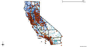
    To give you a visual idea, here’s what the entire California dams layer (red triangles) looks like (zoomed to the extent of the layer, and exported as an image file from QGIS.)

    Dams in CaliforniaDams in California

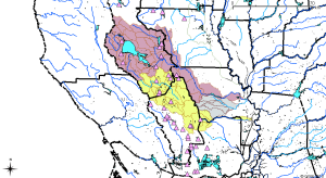
    ..And here’s what it looks like after selecting only the dams (pink triangles) from 4 counties (also zoomed to the extent of the newly created selection):

    Selected dams within 4 counties

    of course in both cases i’ve added background layers like county boundaries and drainage and watersheds of interest.

    Leave a Comment

    specific R tricks

    Barcharts (lattice)

    precip <- barchart(pct_precip_diff ~ date_chunk | emission, groups=model, data=x, horizontal=FALSE, auto.key=list(rectangles=TRUE,columns=3,points=FALSE,cex=0.6),origin=0,ylab=”Precipitation difference (%)”,
    panel=function(x,y,…){
    panel.barchart(x,y,…);
    panel.abline(h=0,lty=2)}

    )

    Reordering factors using transform

    # merge the 2 dataframes which have same headers
    threatdata=merge(x.threat,x.people,all=T)

    #rename column headers
    colnames(threatdata)=c(“Threat”,”Counts”,”ThreatClass”,”Percentage”)
    ###### —- customize from here —————

    threatdata <- transform(threatdata, Threat=factor(Threat, levels=c(‘Extreme threat’, ‘Very High threat’, ‘High threat’, ‘Moderate threat’, ‘Little or no threat’)))

    p <- barchart(Threat~Percentage,groups=ThreatClass, data=threatdata,auto.key=TRUE,xlab=”Percentage of Grid Cell”)

    time series plots using ggplot2

    ##R commands using ggplot2 library
    # temp and precip ts all 6 projections individually marked
    temp.ts=qplot(date,mean_temp,data=x,color=emission,lty=model,geom=c(“path”),xlab=””,ylab=expression(paste(“Avg Annual Temperature (“,degree,”C)”)))
    precip.ts=qplot(date,sum_precip,data=x,color=emission,lty=model,geom=c(“path”),xlab=””,ylab=”Annual Precipitation (mm)”)
    ##
    ##How to get a ribbon plot?temperature
    p <- ggplot(x, aes(x = date, y = mean_temp, colour = emission,fill=emission))
    ppp=p + stat_summary(fun = “range”, geom=”ribbon”)
    temp.tsribbon=ppp + opts(axis.title.x=theme_blank()) + scale_y_continuous(expression(paste(“Avg Annual Temperature (“,degree,”C)”)))
    ####removes x axis label and renames y axis

    Leave a Comment

    oneliners

    ogr2ogr

    Converts from one vector gis format to another; reproject vector gis datasets

    Reprojecting

    ##Example: Tanzania admin to Latlong, WGS84 (EPSG:4326)

    ogr2ogr -f “ESRI Shapefile” -t_srs “EPSG:4326” tzadmin1_LL.shp tzadmn1.shp

    Assign missing projection

    ##Example: assigning projection to final file of district level boundaries:

    ogr2ogr -f “ESRI Shapefile” -a_srs “EPSG:4326” tan_adm.shp

    kml output using ogr2ogr

    http://www.gdal.org/ogr/drv_kml.html

    useful linux utilities

    wget

    extract only particular files buried in folders, and not recreate folders

    #Example: downloading GIMMS global NDVI data at one go

    >wget -r -nd -A .gz ftp://ftp.glcf.umiacs.umd.edu/glcf/GIMMS/Geographic/

    Renaming files

    strip out latter half of file

    file=06feb15a.n17-VIg_data.tif ##
    filename=`basename $file .n17-VIg_data.tif`

    tar

    unzipping tar.gz files

    tar zxfv filename.tar.gz

    scp

    using scp to copy from remote to local machine

    >scp 192.aaa.x.yyy:/data/UrbanProjectionsFromLLNL/extract_urban_pop_starspan.sh Desktop/

    starspan

    Extracting from hundreds of rasters to vector polygons

    # Example: Extracting Avg NDVI for each of 8 Protected areas; dump average NDVI into a csv file

    starspan –vector ../ProtectedAreas-Africa/Tanzania/WDPAEXtractTest_vishal.mehta@sei-us.org3_2_2009222611_PG.shp –raster *.tif –stats ndvistats.csv avg

    Leave a Comment

    kml animation from vector polygons

    About

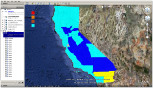
    This one’s about going from GRASS thematic vector polygon data to kml animation that can be viewed on Google Earth. The image is a static screenshot taken from the output Google Earth overlay.

    screenshot-GE

    Input Dataset

    California Population change into 2100. There is one column with 2000 population numbers. Columns pcyyyy refer to population percentage difference from year 2000 to year yyyy.

    v.info -c CountyPop2
    Displaying column types/names for database connection of layer 1:
    INTEGER|cat
    CHARACTER|NAME
    INTEGER|NUM
    CHARACTER|COUNTY
    DOUBLE PRECISION|countynum
    DOUBLE PRECISION|p2000
    DOUBLE PRECISION|pc2010
    DOUBLE PRECISION|pc2015
    DOUBLE PRECISION|pc2020
    DOUBLE PRECISION|pc2025
    DOUBLE PRECISION|pc2030
    DOUBLE PRECISION|pc2035
    DOUBLE PRECISION|pc2040
    DOUBLE PRECISION|pc2045
    DOUBLE PRECISION|pc2050
    DOUBLE PRECISION|pc2055
    DOUBLE PRECISION|pc2060
    DOUBLE PRECISION|pc2065
    DOUBLE PRECISION|pc2070
    DOUBLE PRECISION|pc2075
    DOUBLE PRECISION|pc2080
    DOUBLE PRECISION|pc2085
    DOUBLE PRECISION|pc2090
    DOUBLE PRECISION|pc2100

    The Script

    This shell/GRASS script below can be saved as v.out.kml.sh. Run it using

    sh v.out.kml inputvector outputkml

    #!/bin/bash
    ############################################################################
    # Apr 2009. Script to create
    # a) sequence of GRASS thematic vector displays from one vector dataset, each layer corresponds to a column of the attribute table
    # b) sequence of png images from above thematic vectors
    # b) write images into a kml file for overlay onto Google Earth
    # —-Vishal K. Mehta
    # cmd: sh v.out.kml.sh inputvector outputkmlfilename
    #####################################################################
    #
    # get current region settings from thematic map of interest-input file
    g.region vect=$1
    # Store current environment
    OLD_GRASS_WIDTH=$GRASS_WIDTH
    OLD_GRASS_HEIGHT=$GRASS_HEIGHT
    OLD_GRASS_PNGFILE=$GRASS_PNGFILE
    OLD_GRASS_TRANSPARENT=$GRASS_TRANSPARENT
    OLD_GRASS_TRUECOLOR=$GRASS_TRUECOLOR
    LEGEND_WIDTH=500
    LEGEND_HEIGHT=500
    LEGEND_TEXT_COLOR=white
    BACKGROUND_COLOR=black
    #1. create a legend file
    #d.thematic.area -l map=CountyPop2 column=pc2100 breaks=20,40,60 colors=cyan,brown,orange,red legendfile=popchange.leg
    export GRASS_WIDTH=$LEGEND_WIDTH
    export GRASS_HEIGHT=$LEGEND_HEIGHT
    export GRASS_BACKGROUNDCOLOR=$BACKGROUND_COLOR
    export GRASS_TRANSPARENT=TRUE ##
    export GRASS_TRUECOLOR=TRUE ##
    export GRASS_PNGFILE=legend.png
    d.mon start=PNG
    d.mon select=PNG
    #2. use d.graph on legend file the legend file popchange.leg is created outside of this code
    d.graph input=popchange.leg color=$LEGEND_TEXT_COLOR
    #
    d.mon stop=PNG
    mogrify -transparent black legend.png
    # now display the vector thematic layers
    # define the driver settings
    export GRASS_WIDTH=`g.region -g | grep “cols” | cut -d= -f2`
    export GRASS_HEIGHT=`g.region -g | grep “rows” | cut -d= -f2`
    export GRASS_TRANSPARENT=TRUE ##
    export GRASS_TRUECOLOR=TRUE ##
    yr=2010
    while [ $yr -lt 2105 ] ; do
    echo “yr is $yr ”
    #create png images
    export GRASS_PNGFILE=pc$yr.png
    d.mon start=PNG
    d.mon select=PNG
    d.thematic.area map=$1 column=pc$yr breaks=20,40,60 colors=cyan,blue,yellow,red
    #d.text -b text=”$yr Population” at=50,90 size=4
    d.mon stop=PNG
    # year 2095 column is non-existent so needs to be skipped
    if [ $yr -eq 2090 ]; then yr=$((yr+10)); else yr=$((yr+5)); fi;
    done

    #
    # Create the kml file
    #TITLE=`r.info -m $GIS_OPT_INPUT | cut -d= -f2`
    TITLE=”Population”
    NORTH=`g.region -g | grep -m1 “n=” | cut -d= -f2`
    SOUTH=`g.region -g | grep -m1 “s=” | cut -d= -f2`
    EAST=`g.region -g | grep -m1 “e=” | cut -d= -f2`
    WEST=`g.region -g | grep -m1 “w=” | cut -d= -f2`
    echo “<?xml version=\”1.0\” encoding=\”UTF-8\”?>” > $2.kml
    echo “<kml xmlns=\”http://earth.google.com/kml/2.2\”>” >> $2.kml
    # now begins stack of images
    echo “<Folder>” >> $2.kml
    echo “<open>1</open>” >> $2.kml
    echo “<name>California Population Projections</name>” >> $2.kml
    echo “<description>Percentage difference from 2000 Population</description>” >> $2.kml
    echo “<visibility>1</visibility>” >> $2.kml
    echo “<open>0</open>” >> $2.kml
    # add legend first
    echo “<ScreenOverlay>”  >> $2.kml
    echo “<name>Legend</name>” >> $2.kml
    echo “<Icon>”  >> $2.kml
    echo “<href>legend.png</href>”  >> $2.kml
    echo “</Icon>”  >> $2.kml
    echo “<overlayXY x=\”0\” y=\”1\” xunits=\”fraction\” yunits=\”fraction\”/>”  >> $2.kml
    echo “<screenXY x=\”0.05\” y=\”0.95\” xunits=\”fraction\” yunits=\”fraction\”/>”  >> $2.kml
    echo “<rotationXY x=\”0\” y=\”0\” xunits=\”fraction\” yunits=\”fraction\”/>”  >> $2.kml
    echo “<size x=\”200\” y=\”200\” xunits=\”pixels\” yunits=\”pixels\”/>”  >> $2.kml
    echo “</ScreenOverlay>”  >> $2.kml
    echo “<TimeSpan>” >> $2.kml
    echo “<begin>2010-01</begin>” >> $2.kml
    echo “<end>2100-12</end>” >> $2.kml
    echo “</TimeSpan>” >> $2.kml
    # start loop for sequence of images
    yr=2010
    while [ $yr -lt 2105 ] ; do
    if [ $yr -eq 2090 ]; then endyr=$((yr+10));
    elif [ $yr -eq 2100 ]; then endyr=$((yr));
    else endyr=$((yr+5)); fi;
    echo “<GroundOverlay>” >> $2.kml
    echo “<name>$yr</name>” >> $2.kml
    echo “<visibility>1</visibility>” >> $2.kml
    echo “<drawOrder>1</drawOrder>” >> $2.kml
    echo “<TimeSpan>” >> $2.kml
    echo “<begin>$((yr))-01</begin>” >> $2.kml
    echo “<end>$((endyr))-12</end>” >> $2.kml
    echo “</TimeSpan>” >> $2.kml
    echo “<Icon>” >> $2.kml
    echo “<href>pc$yr.png</href>” >> $2.kml
    echo “</Icon>” >> $2.kml
    echo “<LatLonBox>” >> $2.kml
    echo “<south>$SOUTH</south>” >> $2.kml
    echo “<north>$NORTH</north>” >> $2.kml
    echo “<west>$WEST</west>” >> $2.kml
    echo “<east>$EAST</east>” >> $2.kml
    echo “</LatLonBox>” >> $2.kml
    echo “</GroundOverlay>” >> $2.kml
    if [ $yr -eq 2090 ]; then yr=$((yr+10)); else yr=$((yr+5)); fi;
    done
    #
    echo “</Folder>” >> $2.kml
    echo “</kml>” >> $2.kml
    # Restore the environment
    export GRASS_WIDTH=$OLD_GRASS_WIDTH
    export GRASS_HEIGHT=$OLD_GRASS_HEIGHT
    export GRASS_PNGFILE=$OLD_GRASS_PNGFILE
    export GRASS_TRANSPARENT=$OLD_GRASS_TRANSPARENT
    export GRASS_TRUECOLOR=$OLD_GRASS_TRUECOLOR

    ######END OF SCRIPT#########

    Notes/To Do

    This script is not fully automated. In particular, the legend specs file is hardcoded.Getting a decent legend for GRASS thematic layers is a Major Pain.

    Related posts “thematic maps in GRASS”; “another attempt at animated gif”.

    Acknowledgements

    David Finlayson‘s r.out.kml script, to convert a single GRASS raster to kml.

    Comments (1)

    another attempt at animated gif

    This one was created in Image Magick. It works alright when opened in a web browser. Does it work when uploaded on WordPress??

    another attempt at an animated gif

    WHAT WORKED

    It worked only  by creating a link to the gif file. Not by simply inserting it as an image…

    WHAT IS IT?

    Its an animation every 5 yrs of projected California population data..

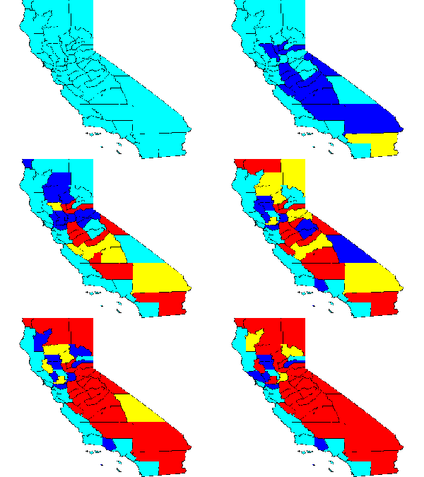
    How was it created?

    First, I had a sequence of .png images, extracted from GRASS GIS work (to be posted later). Then I ran a simple Image Magick utility to take the stack of .png files and create an animated gif called “trial.gif”. Its an endless loop, anda 20/100 second delay between images.

    convert -delay 20 -loop 0 *.png trial.gif

    I learned about this useful command here.

    To Do

    1. The image files must be named in some logical order. For example if they are named file1, file 2….file20, it wont work right. The images will be animated from file1, file10,file11…

    So the files must be renamed correctly…I’m working on it. If you know, please comment!

    2. In GRASS I still need to add a legend and title etc..am working on it

    3. Then I’m going to create a kml animation..

    Leave a Comment

    animated gif

    pastfuture


    About

    This is a simple animated gif of 2 images : of watercolors. One (the happy one:) done by Debbie, the other, apocalyptic one is mine. is one the geologic past, and the other the future? Or vice-versa? it could work either way…

    Shucks…the animated gif works out ok if opened in a browser, but does not seem to work up here..oh well. If anybody know how to make an animated gif work on WordPress let me know..

    What works

    Linking to the animated gif works – because, it opens up a web browser..

    Embedding the image file directly does not work –  this is why the topmost image is not animated on wordpress.

    Notes

    I cant embed a picasa slideshow into WordPress; and I did not like the slideshow options WordPress suggested – they were just cheesy!

    So now i’m playing with GIMP to see if i can just post an animated gif instead. Its a pain though, to be putting up pictures separately likely this..

    Leave a Comment

    flowers in springtime

    spring flowers blooming in our front and backyards here in Davis, CA!

    spring flowers in our garden

    spring flowers in our garden

    Leave a Comment

    geodata for guadiana, spain

    Lower Guadiana basin, Spain

    This is my work area on geodata collection for Guadiana, Spain. In support of visiting scholar Irene Blanco

    ####Soils

    ###Sources

    1. European Soils Database

    Link:http://eusoils.jrc.ec.europa.eu/data.html
    Resolution:
    Format: vector; also raster files of 70+ properties in ESRI GRID format, Lambert Azimuthal coordinates;
    Issues:
    Status: pending;

    ####Rivers

    ###Sources

    1. Hydro1K dataset for Europe

    Link:http://edc.usgs.gov/products/elevation/gtopo30/hydro/eu_streams.html
    Resolution: NA
    Format: shapefile
    Issues: This is based on flow accumulation analysis on GTOPO elevation data
    Status: archive downloaded. unprocessed.

    2. Digital Chart of the World

    Link:http://www.maproom.psu.edu/dcw/
    Resolution: NA
    Format: arc info format (.eoo);Latlong Clarke1866
    Issues: must be reprojected; dataset is old
    Status: selected archive for Spain downloaded – drainage, also landcover, roads, populated places. unprocessed
    Scripts:
    #converting the drainage into shapefiles and also reprojecting to wgs84
    ogr2ogr -f “ESRI Shapefile” -t_SRS EPSG:4326 DCW_drainage dnnet.e00
    <ERROR 6: Can’t create fields of type IntegerList on shapefile layers.>
    what is this?? try importing directly in Manifold/Arcview/ArcGIS

    3.

    http://dataservice.eea.europa.eu/dataservice/metadetails.asp?id=1053

    4. European Commission Joint Research Center

    Link:http://desert.jrc.ec.europa.eu/action/php/index.php?action=view&id=24
    Resolution:NA
    Format: Latlongwgs84; ESRI ArcGIS geodatabase; cannot use in GRASS, must switch to ArcGIS
    Issues: archive downloaded for “SouthWest” tile which includes Spain. unprocessed; handover to Irene to continue in ArcGIS.

    ####DEM

    ###Sources

    1. GTOPO30

    Link:http://eros.usgs.gov/products/elevation/gtopo30/gtopo30.html
    Resolution: 30 arc seconds (~1km)
    Format: Binary, 16bit integer, Motorola MSB
    Issues: Failed to import using several software; 2 tiles needed to cover lower Guadiana basin
    Status: 2 tiles raw data downloaded, unprocessed

    2. SRTM

    Link:http://eros.usgs.gov/products/elevation/gtopo30/gtopo30.html
    Resolution: 3 arc seconds (~90m)
    Format: SRTM DEM format
    Issues: Will need 20-30 tiles downloaded, imported and mosaiced
    Status: 2 tiles raw data downloaded by Irene; unprocessed; abandoned for – no need for such high resolution for WEAP work

    3. GLOBEDEM

    Link:http://www.ngdc.noaa.gov/mgg/topo/
    Resolution: 30 arc seconds (~1km)
    Format: Binary, 16bit integer, Motorola MSB
    Issues: Boundary coordinates fed to download rectangular region for most of Spain
    Status: Successfully processed in GRASS; and also output to ESRI Ascii grid format which can be used in ArcGIS and Arcview.
    Scripts:
    ###GRASS GIS
    ##March 31 Guadiana basin DEM work
    #import GlobeDEM using r.in.bin (http://grass.itc.it/gdp/html_grass63/r.in.bin.html)
    #r.in.gdal did not work

    r.in.bin -sb input=Vishal_Guadiana.bin output=GlobeDEM north=44.0 south=35.9 east=2.0 west=-9.3 r=972 c=1356 bytes=2 anull=-500

    # creating watershed at 1000km2 threshold
    r.watershed GlobeDEM thresh=1000 accum=FlowAccum1000 drain=draindir1000 basin=basin_1000 stream=rivers1000

    #creating and displaying shaded relief
    r.shaded.relief GlobeDEM shadedmap=GlobeShaded
    d.his h=elevation i=GlobeShaded

    # clean up border bad watersheds
    r.mapcalc basins=basin_1000

    r.null map=basins setnull=98,100,102,104,106,108,110,112,114,116,118,120,662,660,798,1082,800,802,1078,804,936,944,1060,1068,1072,1100,1106,1110,1114,1118,1122,1126,1130,1166,1168,1170

    r.null map=basins setnull=4,6,8,10,12,14,16,20,22,24,26,28,30,416,414,640,644,648,652,650,656,654

    # convert basins to vector
    r.to.vect -s basins out=basins feature=area
    #display vector watersheds map
    d.vect -c basins
    #export to shapefile; -ep flags generate .prj and convert lines to polygons respectively.
    v.out.ogr -ep input=basins type=area dsn=Watersheds.shp format=ESRI_Shapefile
    v.info basins

    # convert GlobeDEM into Esri Ascii grid; also the partially cleaned up ‘basins’ watersheds raster layer. the basins will need to be converted to vector and cleaned up later in Manifold/Arcview or ArcGIS
    r.out.gdal format=AAIGrid input=GlobeDEM output=GlobeDEM.asc nodata=-9999
    r.out.gdal format=AAIGrid input=basins output=basins.asc nodata=-9999
    #

    Leave a Comment

    Older Posts »